Project Tutorial: Predicting Tech Salaries with Machine Learning Using the 2023 Stack Overflow Developer Survey (Part 2 of 2)

In Part 1 of this series, we turned 48,000 rows of messy survey data into a clean, fully numeric dataset with 75 features and 14,924 rows. We dropped columns, filtered outliers, encoded categorical variables, and engineered binary skill features for languages, databases, cloud platforms, and DevOps tools.
Now it's time to build the model and see what the data actually tells us.
In Part 2, we'll check for multicollinearity, train a linear regression model, evaluate how well it performs across different salary ranges, and interpret the coefficients to extract concrete, actionable insights about what actually influences developer salaries.
What You'll Learn
By the end of Part 2, you'll know how to:
- Identify and address multicollinearity before training
- Train and evaluate a linear regression model with scikit-learn
- Use R² and MAE to assess model performance
- Read residual plots to diagnose model weaknesses
- Interpret regression coefficients as real-dollar salary impacts
- Communicate data-driven findings to a non-technical audience
Before You Start
This tutorial picks up directly from Part 1. Make sure you've either completed that walkthrough or reviewed the solution notebook on GitHub before continuing. You can also access the full project in the Dataquest app.
Your Python environment should have pandas, scikit-learn, matplotlib, and seaborn installed.
Step 1: Checking Correlations with Salary
We'll start by separating our features (X) from our target variable (y) and then calculating how each feature correlates with salary.
X = df_model.drop(columns=['ConvertedCompYearly'])
y = df_model['ConvertedCompYearly']

print(f"Features shape: {X.shape}")
print(f"Target shape: {y.shape}")

correlations = X.corrwith(y).sort_values(ascending=False)
print("\n=== TOP 20 POSITIVE CORRELATIONS WITH SALARY ===")
print(correlations.head(20))
print("\n=== TOP 20 NEGATIVE CORRELATIONS WITH SALARY ===")
print(correlations.tail(20))
Features shape: (14924, 75)
Target shape: (14924,)
=== TOP 20 POSITIVE CORRELATIONS WITH SALARY ===
Country_United States of America 0.600111
YearsCodePro 0.310453
WorkExp 0.305963
YearsCode 0.302707
Age_Ordinal 0.258526
OrgSize_Ordinal 0.211776
Has_Terraform 0.175568
RemoteWork_Remote 0.142808
Has_AWS 0.140094
Has_Kubernetes 0.126078
Has_Go 0.121580
DevType_Engineering manager 0.106681
DevType_Senior Executive (C-Suite, VP, etc.) 0.097640
Has_Rust 0.085012
Has_Python 0.083086
Has_React 0.063394
Has_Docker 0.061214
Industry_Financial Services 0.060895
Has_Redis 0.058601
Country_Switzerland 0.057682
dtype: float64
=== TOP 20 NEGATIVE CORRELATIONS WITH SALARY ===
...
Country_Brazil -0.132113
Country_India -0.181109
Country_Other -0.277522
dtype: float64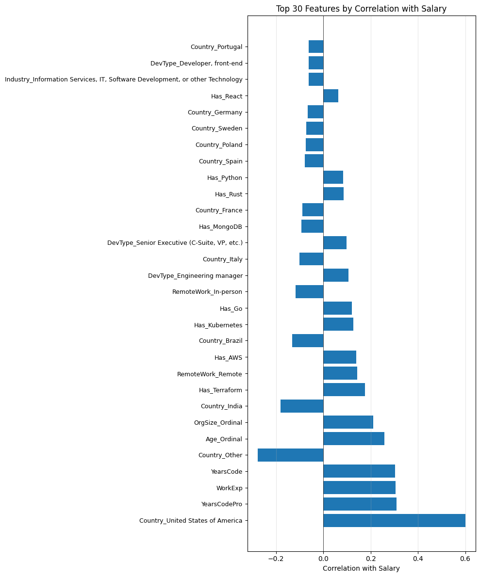
When we visualize this data, a few things jump out immediately. Being based in the U.S. has by far the strongest positive correlation with salary at 60%. And toward the bottom, we see strong negative correlations for countries like India, Brazil, and "Other" (the catch-all for countries outside the top 15). Country is clearly doing a lot of work in this dataset.
We also notice something worth pausing on: YearsCodePro, WorkExp, YearsCode, and Age_Ordinal all show correlations around 25-31%. That's a red flag for multicollinearity, and we need to address it before training.
Step 2: Checking for Multicollinearity
Multicollinearity happens when two or more features in your dataset measure essentially the same thing. When that's the case, they effectively double-count the same information and can distort the model's coefficient estimates.
top_20_features = correlations.abs().sort_values(ascending=False).head(20).index.tolist()
feature_corr = X[top_20_features].corr()

high_corr_pairs = []
for i in range(len(feature_corr.columns)):
    for j in range(i+1, len(feature_corr.columns)):
        if abs(feature_corr.iloc[i, j]) > 0.8:
            high_corr_pairs.append((feature_corr.columns[i], feature_corr.columns[j], feature_corr.iloc[i, j]))

print("\nHighly correlated feature pairs (>0.8):")
for feat1, feat2, corr in high_corr_pairs:
    print(f"  {feat1} <-> {feat2}: {corr:.3f}")
Highly correlated feature pairs (>0.8):
YearsCodePro <-> WorkExp: 0.929
YearsCodePro <-> YearsCode: 0.906
YearsCodePro <-> Age_Ordinal: 0.801
WorkExp <-> YearsCode: 0.861
WorkExp <-> Age_Ordinal: 0.827There it is. YearsCodePro, WorkExp, YearsCode, and Age_Ordinal are all highly correlated with each other, which makes sense: the more years of experience you have, the older you tend to be. Keeping all four in the model would give "years of experience" four times the influence it deserves.
The fix is to keep the most informative one and drop the rest. We keep YearsCodePro (professional coding experience) as our single experience signal, since it's most directly tied to salary, and drop the other three.
multicollinear_drops = ['YearsCode', 'WorkExp', 'Age_Ordinal']
X_reduced = X.drop(columns=multicollinear_drops)
print(f"Shape after dropping multicollinear features: {X_reduced.shape}")
Shape after dropping multicollinear features: (14924, 72)Learning Insight: Which columns you drop here is a judgment call. We kept
YearsCodeProbecause it most directly measures professional experience. You could just as reasonably argue forWorkExp. If you're extending this project, try keeping different combinations and see how the model's R² changes. These kinds of experiments are exactly what make a project worth showcasing.
We also take the opportunity to drop any features with nearly zero correlation with salary (absolute correlation below 0.01), since they add noise without contributing signal.
weak_features = correlations_reduced[abs(correlations_reduced) < 0.01].index.tolist()
print(f"\n=== Features with correlation < 0.01: {len(weak_features)} ===")
print(weak_features)

X_final = X_reduced.drop(columns=weak_features)
print(f"\n=== FINAL FEATURE SET ===")
print(f"Features: {X_final.shape[1]}")
print(f"Rows: {X_final.shape[0]}")
=== Features with correlation < 0.01: 4 ===
['Has_SQL', 'Industry_Retail and Consumer Services', 'DevType_DevOps specialist', 'Industry_Legal Services']
=== FINAL FEATURE SET ===
Features: 68
Rows: 14924Four features dropped, leaving us with a final set of 68 features to train on.
Step 3: Training the Model
With our feature set finalized, we're ready to build the model. We'll use scikit-learn's LinearRegression, split the data 80/20 into training and test sets, and evaluate performance on both.
X = df_final.drop(columns=['ConvertedCompYearly'])
y = df_final['ConvertedCompYearly']

X_train, X_test, y_train, y_test = train_test_split(
    X, y, test_size=0.2, random_state=42
)

print(f"Training set: {X_train.shape}")
print(f"Test set: {X_test.shape}")

model = LinearRegression()
model.fit(X_train, y_train)

y_pred_train = model.predict(X_train)
y_pred_test = model.predict(X_test)
Training set: (11939, 68)
Test set: (2985, 68)Those four lines are the entire modeling pipeline. Under the hood, scikit-learn is fitting a line through 68-dimensional space by minimizing the sum of squared errors, but from our perspective it's a clean three-step process: create the object, fit it to training data, and generate predictions.
Now let's see how it performed.
print("\n=== MODEL PERFORMANCE ===")
print("\nTraining Set:")
print(f"R² Score: {r2_score(y_train, y_pred_train):.4f}")
print(f"MAE: ${mean_absolute_error(y_train, y_pred_train):,.2f}")

print("\nTest Set:")
print(f"R² Score: {r2_score(y_test, y_pred_test):.4f}")
print(f"MAE: ${mean_absolute_error(y_test, y_pred_test):,.2f}")
=== MODEL PERFORMANCE ===
Training Set:
R² Score: 0.5531
MAE: $29,834.58
Test Set:
R² Score: 0.5647
MAE: $30,881.92Our model explains about 55-56% of the variance in salary (R²), with a mean absolute error of roughly \$30,000. That means on average, the model's predictions are off by around \$30k.
Whether that's "good" depends on context. On one hand, salary is notoriously hard to predict from survey data alone. There are factors like negotiation, company-specific pay scales, and equity compensation that a survey simply can't capture. On the other hand, \$30k is a meaningful margin if someone is relying on this for career planning.
The more reassuring finding is that our training and test scores are nearly identical. An R² of 55% training vs. 56% test means the model is generalizing well and isn't just memorizing the training data (overfitting). That's a sign we built a clean, well-regularized feature set.
Learning Insight: A common beginner mistake is to optimize entirely for a high R² on training data. If training R² is 95% but test R² is 55%, your model has memorized the training examples and will perform poorly on anything new. The goal is always for training and test scores to be close together, even if both are modest.
Step 4: Diagnosing the Model with Residual Plots
Before jumping to interpretation, let's check whether linear regression is actually a good fit for this problem.
plt.figure(figsize=(12, 5))

plt.subplot(1, 2, 1)
plt.scatter(y_test, y_pred_test, alpha=0.5)
plt.plot([y_test.min(), y_test.max()], [y_test.min(), y_test.max()], 'r--', lw=2)
plt.xlabel('Actual Salary ($)')
plt.ylabel('Predicted Salary ($)')
plt.title('Predicted vs Actual Salaries (Test Set)')
plt.grid(alpha=0.3)

plt.subplot(1, 2, 2)
residuals = y_test - y_pred_test
plt.scatter(y_pred_test, residuals, alpha=0.5)
plt.axhline(y=0, color='r', linestyle='--', lw=2)
plt.xlabel('Predicted Salary ($)')
plt.ylabel('Residuals ($)')
plt.title('Residual Plot')
plt.grid(alpha=0.3)

plt.tight_layout()
plt.show()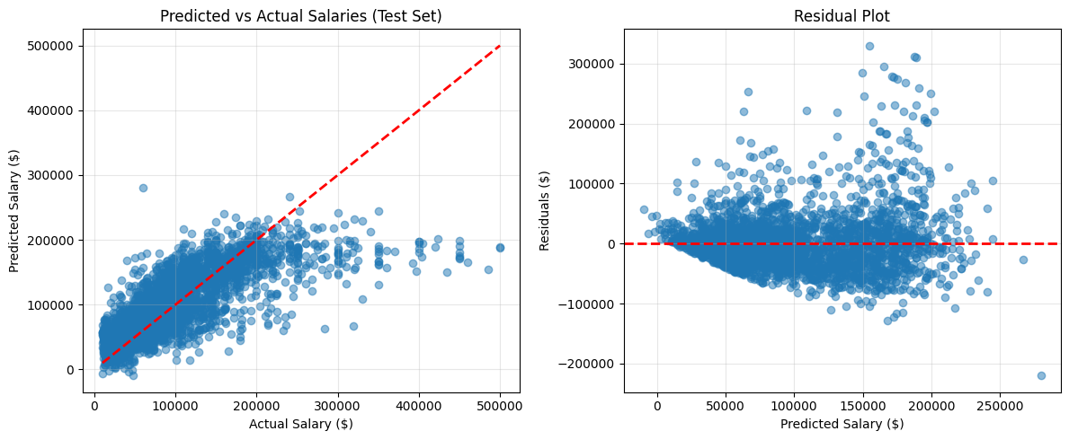
The predicted vs. actual plot shows that for low and mid-range salaries, the model tracks well along the diagonal. But as actual salaries get higher, predictions start lagging significantly behind. The model consistently underestimates high earners.
The residual plot (right side) shows residuals spreading wider as predicted salary increases. In a well-behaved linear model, residuals would be randomly scattered around zero with roughly equal spread throughout. The widening fan shape here tells us the model's errors are larger for higher-paid developers.
We'll explore exactly where the model breaks down next.
Step 5: Evaluating Performance by Salary Range
Let's quantify what we're seeing in those charts by bucketing predictions into salary ranges.
salary_ranges = pd.DataFrame({
    'Actual': y_test,
    'Predicted': y_pred_test,
    'Error': abs(y_test - y_pred_test)
})
salary_ranges['Salary_Range'] = pd.cut(salary_ranges['Actual'],
                                        bins=[0, 50000, 100000, 150000, 200000, 500000],
                                        labels=['<$50k', '$50-100k', '$100-150k', '$150-200k', '>$200k'])

print("=== ERROR BY SALARY RANGE ===")
error_by_range = salary_ranges.groupby('Salary_Range')['Error'].agg(['mean', 'median', 'count'])
print(error_by_range)
=== ERROR BY SALARY RANGE ===
mean median count
Salary_Range
<$50k 23094.124364 19159.462266 743
$50-100k 22427.082209 16700.085894 1099
$100-150k 30620.128394 26940.220831 593
$150-200k 27475.614914 20436.613767 318
>$200k 101212.327040 84484.124508 232The pattern is stark. For developers earning under \$150k, mean absolute error stays in the \$22-31k range, which is workable. But for earners above \$200k, the average error jumps to \$101k, and the median error is \$84k. The model is effectively off by about half for high earners.
Two factors explain this. First, high earners are a small group: only 232 people in the test set earn more than \$200k. With limited training examples in that range, the model doesn't have enough signal to learn their patterns well. Second, high-salary roles often involve factors like equity compensation, FAANG-level pay bands, or unique seniority arrangements that simply aren't captured anywhere in the survey.
A promising next step would be to train separate models for different salary brackets, keeping the low-to-mid model as-is and using a different approach (like a Random Forest) for the high-earner segment.
Step 6: Interpreting the Coefficients
R² and MAE tell us how well the model predicts. Coefficients tell us what it learned. Let's dig into those now.
coefficients = pd.DataFrame({
    'Feature': X.columns,
    'Coefficient': model.coef_
})
coefficients['Abs_Coefficient'] = abs(coefficients['Coefficient'])

coefficients_sorted = coefficients.sort_values('Coefficient', ascending=False)

print("\n=== TOP 20 POSITIVE COEFFICIENTS (Increase Salary) ===")
print(coefficients_sorted.head(20)[['Feature', 'Coefficient']].to_string(index=False))
print("\n=== TOP 20 NEGATIVE COEFFICIENTS (Decrease Salary) ===")
print(coefficients_sorted.tail(20)[['Feature', 'Coefficient']].to_string(index=False))
=== TOP 20 POSITIVE COEFFICIENTS (Increase Salary) ===
Feature Coefficient
Country_United States of America 56311.330286
DevType_Senior Executive (C-Suite, VP, etc.) 35917.362070
Country_Switzerland 29827.786692
DevType_Engineering manager 24117.744900
DevType_Other (please specify): 13231.239000
DevType_Developer, mobile 12666.293949
Has_Terraform 8671.813906
Industry_Financial Services 7478.518615
Has_Rust 6580.300282
Has_Kubernetes 6533.803807
DevType_Other 6352.495143
Has_TypeScript 6326.088629
Has_Go 6004.289804
Has_React 5754.080078
DevType_Developer, back-end 5077.897084
Has_AWS 4984.284478
Has_Kotlin 4632.116174
OrgSize_Ordinal 4471.811309
Has_Redis 3408.064819
RemoteWork_Remote 3080.409892
=== TOP 20 NEGATIVE COEFFICIENTS (Decrease Salary) ===
Feature Coefficient
Industry_Insurance -6709.806111
Has_CSharp -7105.670401
Has_SpringBoot -7286.369380
Country_United Kingdom of Great Britain and Northern Ireland -9496.742854
Employment_Simple_Full-time + Freelance -12568.844850
Industry_Wholesale -16399.784485
Country_Germany -17270.165382
Employment_Simple_Full-time -18322.343972
Country_Netherlands -19257.820041
Industry_Higher Education -22416.839984
Employment_Simple_Part-time -30028.069466
Country_Other -31984.032445
Country_France -35248.270299
Country_Sweden -35394.571760
Country_Poland -37272.735270
Country_Spain -37908.859947
Country_Portugal -39461.936394
Country_Italy -45739.032413
Country_Brazil -57285.162776
Country_India -61208.113364The top 10 most impactful features are almost entirely country-based. Being located in the U.S. is associated with a \$56k salary premium (relative to our reference group), while being in India is associated with a \$61k reduction. Switzerland, with its high cost of living and strong finance and pharma sector, shows a \$30k premium.
Country is the single biggest lever in this model, but it's also the one factor most developers can't easily change. Let's look at what they can.
Let's also break down average impact by feature category to understand the relative weight of each group.
country_coefs = coefficients[coefficients['Feature'].str.startswith('Country_')]
skill_coefs = coefficients[coefficients['Feature'].str.startswith('Has_')]
devtype_coefs = coefficients[coefficients['Feature'].str.startswith('DevType_')]
industry_coefs = coefficients[coefficients['Feature'].str.startswith('Industry_')]

print(f"Country features - Average absolute impact:  ${country_coefs['Abs_Coefficient'].mean():,.2f}")
print(f"Skill features - Average absolute impact:    ${skill_coefs['Abs_Coefficient'].mean():,.2f}")
print(f"DevType features - Average absolute impact:  ${devtype_coefs['Abs_Coefficient'].mean():,.2f}")
print(f"Industry features - Average absolute impact: ${industry_coefs['Abs_Coefficient'].mean():,.2f}")
Country features - Average absolute impact: $34,265.48
Skill features - Average absolute impact: $3,994.12
DevType features - Average absolute impact: $11,667.53
Industry features - Average absolute impact: $7,721.10Country features have an average absolute impact of \$34k, nearly triple the next category (developer type at \$12k). Skills individually contribute an average of about \$4k each, which is modest but adds up when you combine several.
Step 7: What Can You Actually Control?
Let's filter down to the factors a developer can realistically influence: skills, developer type, experience, organization size, and work arrangement.
controllable_features = coefficients[
    (coefficients['Feature'].str.startswith('Has_')) |
    (coefficients['Feature'].str.startswith('DevType_')) |
    (coefficients['Feature'] == 'YearsCodePro') |
    (coefficients['Feature'] == 'OrgSize_Ordinal') |
    (coefficients['Feature'].str.startswith('RemoteWork_'))
].copy()

controllable_features = controllable_features.sort_values('Coefficient', ascending=False)

print("\n=== FACTORS YOU CAN CONTROL ===")
print("\nTop 15 ways to increase your salary:")
print(controllable_features.head(15)[['Feature', 'Coefficient']].to_string(index=False))
=== FACTORS YOU CAN CONTROL ===
Top 15 ways to increase your salary:
Feature Coefficient
DevType_Senior Executive (C-Suite, VP, etc.) 35917.362070
DevType_Engineering manager 24117.744900
DevType_Other (please specify): 13231.239000
DevType_Developer, mobile 12666.293949
Has_Terraform 8671.813906
Has_Rust 6580.300282
Has_Kubernetes 6533.803807
DevType_Other 6352.495143
Has_TypeScript 6326.088629
Has_Go 6004.289804
Has_React 5754.080078
DevType_Developer, back-end 5077.897084
Has_AWS 4984.284478
Has_Kotlin 4632.116174
OrgSize_Ordinal 4471.811309This is the most practically useful output from the entire project. Here's what the model is telling us:
Role matters most. C-suite positions show a \$36k premium and engineering management a \$24k premium. Mobile developers show a \$13k premium over the baseline. Back-end developers also trend positively.
Cloud and infrastructure skills are the highest-value technical skills. Terraform (\$8.7k), Kubernetes (\$6.5k), and AWS (\$5k) show the strongest positive coefficients among the Has_ features. These tools tend to cluster in senior DevOps and platform engineering roles, which likely explains some of the correlation.
Certain languages carry a meaningful premium. Rust (\$6.6k), Go (\$6k), TypeScript (\$6.3k), and Kotlin (\$4.6k) all show positive coefficients. These tend to be languages that developers specialize in later in their career, after building a strong foundation, which probably also contributes to the signal.
Larger organizations pay more. Each step up in OrgSize_Ordinal is associated with a \$4.5k increase, consistent with the general finding that enterprise and large tech companies offer higher base salaries.
Remote work has a modest positive signal. About \$3k associated with remote work, though this likely reflects that remote-friendly companies (often U.S.-based tech firms) also tend to pay more.
Learning Insight: Correlation in model coefficients doesn't mean "learn Terraform and your salary will increase by \$8,671." It means that, across our dataset, people who use Terraform tend to earn about \$8.7k more than otherwise similar developers who don't. Those developers also likely have more years of experience, work at larger companies, and hold senior roles. Coefficients capture association, not causation. That nuance matters a lot when communicating findings to stakeholders.
Model Summary
Here's a quick look at a few sample predictions to ground the numbers:
sample_idx = [0, 100, 500, 1000, 2000]
comparison = pd.DataFrame({
    'Actual': y_test.iloc[sample_idx].values,
    'Predicted': y_pred_test[sample_idx],
    'Difference': y_test.iloc[sample_idx].values - y_pred_test[sample_idx]
})
print(comparison.to_string(index=False))
Actual Predicted Difference
42167.0 65642.953943 -23475.953943
87813.0 92422.205473 -4609.205473
190000.0 198285.695497 -8285.695497
107090.0 91056.166442 16033.833558
300000.0 241048.205597 58951.794403The model does well for mid-range salaries (rows 2, 3, and 4) but overshoots for the \$42k case and significantly undershoots for the \$300k case, consistent with everything we saw in the residual plots.
What the model does well:
- Explains 56.5% of salary variance
- No overfitting (training and test scores are nearly identical)
- Reasonably accurate for salaries under \$150k (mean error ~\$27-30k)
- Produces interpretable, actionable coefficients
Where it falls short:
- Mean error of \$101k for salaries above \$200k
- Geography dominates and may mask other signals
- Linear assumptions can't capture interactions between features (e.g., Python + ML specialization + senior title)
Limitations Worth Acknowledging
If you're presenting this project in an interview or portfolio, be upfront about a few things.
We dropped roughly 66% of our original data by removing any row with missing values. That's a pragmatic choice given our timeline, but it almost certainly introduced some selection bias. People who fill out a survey completely may differ systematically from people who leave fields blank.
Our \$500k salary cap was also somewhat arbitrary. Some of the salaries above that threshold may be real (think senior engineers at FAANG companies), and excluding them means our model doesn't learn patterns for that segment at all.
Finally, "USA" is a single binary variable, but the salary gap between a developer in rural Iowa and one in San Francisco is enormous. Geographic granularity at the city or region level would almost certainly improve predictions substantially.
Next Steps
There's a lot of room to take this project further:
Try a Random Forest Regressor. Random forests can capture non-linear relationships and interactions between features that linear regression can't. This is the single improvement most likely to meaningfully boost R².
Experiment with feature engineering. Interaction terms (e.g., Has_Kotlin × DevType_Developer_mobile) might give the model better signal for role-specific skill combinations. The difference between YearsCode and YearsCodePro could also serve as a useful "hobbyist time" feature.
Build separate models by salary range. Given how clearly the model breaks down above \$200k, a two-model approach (one for <\$150k, one for >\$150k using a more flexible algorithm) is likely to improve overall accuracy.
Add missing indicators. Rather than dropping rows with null values, you could impute them and add a binary column flagging which values were imputed. This preserves more data while signaling to the model that those values are uncertain.
Resources
- Part 1 of this tutorial
- Solution notebook on GitHub
- Dataquest project in the app
- Machine Learning in Python course
- Dataquest Community Forum
If you take this project further, share it in the community and tag @Anna_strahl. There are a lot of interesting directions this can go, and the community is a great place to get feedback and see what others are building.
Want to read more?
Check out the full article on the original site